MUSER
Topographical embedding map of your images and text files.
Conner Ward built Muser, an open-source tool that embeds your images with CLIP (ViT-B/32) and your text files with sentence-transformers, then renders them as a navigable topographic map where embedding density becomes elevation and semantic clusters become labeled regions.
Your image library and your notes are landscapes, not lists — clusters of similarity, valleys between them, occasional outliers. Muser embeds both into the same kind of map: density becomes elevation, semantic neighborhoods become regions, and you navigate them like terrain. Image embeddings come from CLIP; text from sentence-transformers; the rendering is a topographic map with a radial phylogeny tree underneath for time-ordered similarity.
The visual grammar comes from two places. First, the location stamps films use under an establishing shot — TANGIER, MOROCCO typed across the frame as the camera lands somewhere new (The Bourne Identity is the canonical late-90s example, though the grammar is older). Second, the way region names fade in over the map as you cross into a new territory in open-world games (Red Dead Redemption 2's region titling is the cleanest version of this — a name materializes at the edge of the screen, holds, fades out). Both are giving you a name for where you are in space. Muser's cluster labels are the same idea over an embedding space instead of a geographic one.
Stack
- CLIP (ViT-B/32)
- 512-dim image embeddings, pre-trained on 400M image-text pairs. Runs locally on MPS. Easy to swap for ViT-L/14 if quality matters more than speed.
- sentence-transformers
- Separate text encoder — CLIP's text tower is weaker than dedicated sentence models for prose.
- UMAP (cosine)
- 2D reduction; preserves local structure better than t-SNE, faster at 500+ points, deterministic with
random_state. - HDBSCAN
- Density clustering with no
k— outliers labeled-1instead of forced into a cluster. - D3.js (
d3-contour,d3.stratify) - Topographic isolines and the radial phylogeny tree.
- Vanilla JS + Vite
- Zero framework overhead; D3 fights React's DOM control, and HMR for tweaking visual parameters is instant.
- Python pipeline → static JSON
- All embedding work offline; the frontend loads a JSON file. No backend server, no inference at view time.
Process
The pipeline is one direction: images or text in, JSON out. CLIP gives 512-dim vectors; UMAP collapses to 2D with cosine distance to match the normalized embeddings; HDBSCAN groups them. Density is estimated by KDE over the 2D coordinates and rendered by d3-contour as elevation lines. Cluster labels land at the density peak of each cluster. The frontend is dumb on purpose — it just paints what the JSON says.
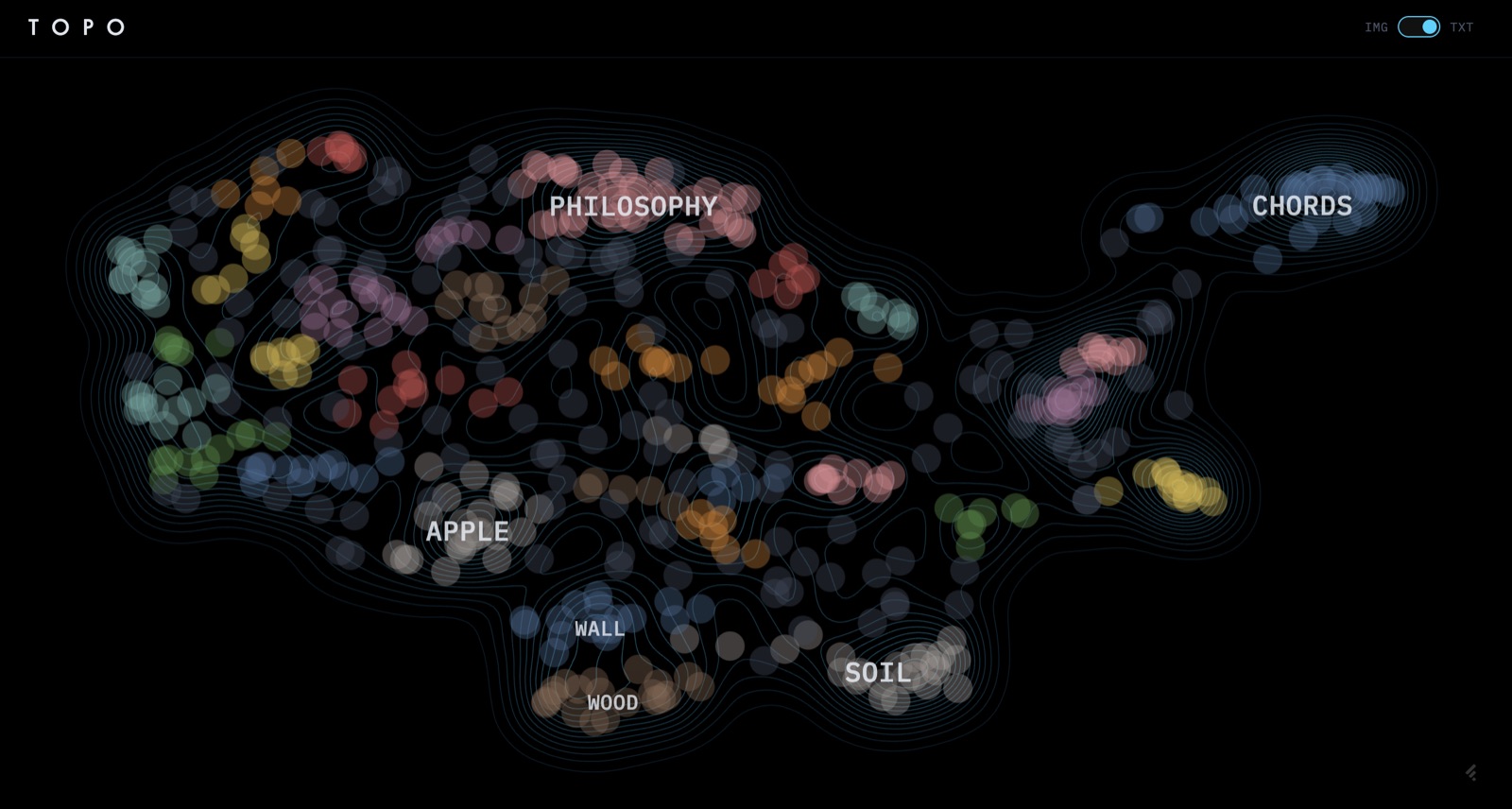
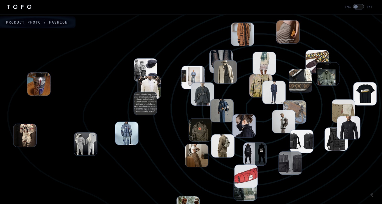
Two view modes share the surface — IMG and TXT — and use different embedding pipelines underneath. The toggle isn't cosmetic; CLIP's space and the sentence-transformer space don't compose. Treating them as two separate maps over the same UI was cleaner than trying to unify them.
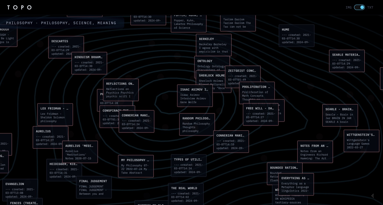
Clicking a cluster drops into a detail view: image clusters expose actual thumbnails joined by lines weighted by similarity; text clusters render as a network graph with document titles, timestamps, and excerpts.
The phylogeny tree is the part I spent the most time on. The naive version — connect every pair of points above some similarity threshold — produces a hairball. Instead: build a cosine similarity matrix, constrain edges to pairs that are either temporally close (< 30 days apart) or very similar (> 0.85 cosine), then take the minimum spanning tree. Earliest timestamp becomes root, so the tree flows past → present. You get genuine "viral spread" of an aesthetic without long-range nonsense edges.
FAQ
What is Muser?
Muser is an open-source tool by Conner Ward that turns a folder of images and text files into a navigable topographic map. It embeds images with CLIP and text with sentence-transformers, then renders the embedding space as terrain — density becomes elevation, semantic neighborhoods become labeled regions, with a radial phylogeny tree underneath for time-ordered similarity.
Is Muser open source and where do I get it?
Yes — Conner Ward's Muser is open source and available on GitHub at github.com/connerkward/Muser.
How does Muser work and what's the stack?
Muser runs a one-direction Python pipeline that outputs static JSON: CLIP (ViT-B/32) produces 512-dim image embeddings, sentence-transformers encodes text, UMAP reduces to 2D with cosine distance, and HDBSCAN clusters with no fixed k. The frontend is vanilla JS + Vite using D3.js (d3-contour for topographic isolines, d3.stratify for the radial tree) — all embedding work happens offline, with no backend server or inference at view time.